msm_demo_minimal
It is a 1D MSM demo code to check the force error calculations with the expected values. In this minimal code, there is no restriction and prolongation steps as it is one level MSM.
Contents
Initialization
I first get rid of old variables and figures.
clear variables
clc
close all
Setting random seed to recreate the results.
s = RandStream('mt19937ar','Seed',7); RandStream.setGlobalStream(s);
Grid spacing is set to h=2.5 to mimic large water sphere.
h = 2.5;
The number of particles.
n=41;
The distribution of the particles on a line. I choose the boundaries -50 and 50 and the n=41 to mimic the large water sphere data in the NAMD-lite. In that data, there are 30006 atoms in a sphere with radius r=44A. The number of atoms in each direction is approximately 2*r/((4/3*pi*r^3/30006)^(1/3)) = 38. I set n=41 in order to locate each particles on the grid with h=2.5. In this way, I am sure that there is no error in anterpolation.
x0 = linspace(-50,50,n);
%x0 = sort(100*rand(n,1)-50);
I take all the masses one. I don't know if this effects my calculations.
q0 = ones(n,1);
Since I know h=2.5 and the boundaries of [-50 50], I can preallocate the finest mesh beforehand. I enlarge the boundary by 2*h on each side.
x1 = linspace(-55,55,45);
The cutoff values that I try. In the dissertation, a=6:20 is used almost always. But here I want to see what happens outside of that safe region.
arange = [1:10 20:10:100 200:100:1000];
This is the C3 Taylor smoothing and its derivative.
s  = @(p) 1 + (p*p-1)*(-1/2 + (p*p-1)*(3/8 + (p*p-1)*(-5 /16)));
sd = @(p)     (2*p)  *(-1/2 + (p*p-1)*(3/4 + (p*p-1)*(-15/16)));
The cubic "numerical" Hermite nodal base and its derivative. The enumeration of the pieces of the functions is as follows:
<--------|--------|--------|--------|--------|------->
        -2       -1        0        1        2
             c1       c2       c3        c4
             c1d      c2d      c3d       c4d --> derivatives
To make sure, I don't make any mistake, I took the functions definitions directlt from NAMD-Lite. However, in NAMD-Lite the enumeration of the pieces are little different.
Enumeration of the cubic pieces in the NAMD-Lite:
<--------|--------|--------|--------|--------|------->
        -2       -1        0        1        2
            phi3     phi2     phi1     phi0
           dphi3    dphi2    dphi1    dphi0 --> derivatives
c1 = @(t) 0.5 * (1 + t) * (2 + t) * (2 + t); % phi3 in NAMD-Lite c1d = @(t) (1.5 * t + 2) * (2 + t); % dphi3 in NAMD-Lite c2 = @(t) (1 + t) * (1 - t - 1.5 * t * t); % phi2 in NAMD-Lite c2d = @(t) (-5 - 4.5 * t) * t; % dphi2 in NAMD-Lite c3 = @(t) (1 - t) * (1 + t - 1.5 * t * t); % phi1 in NAMD-Lite c3d = @(t) (-5 + 4.5 * t) * t ; % dphi1 in NAMD-Lite c4 = @(t) 0.5 * (1 - t) * (2 - t) * (2 - t); % phi0 in NAMD-Lite c4d = @(t) (1.5 * t - 2) * (2 - t) ; % dphi0 in NAMD-Lite
Direct calculation
In the following double loop, I create the original kernel matrix and calculate the exact forces.
G = zeros(n,n);
freal = zeros(n,1);
for i=1:n-1
    for j=i+1:n
        rij = x0(i)-x0(j);
        r = abs(rij);
        r_1 = 1/r;
        rij_r3 = q0(i)*q0(j)*rij/r^3;

        G(i,j) = r_1;
        G(j,i) = G(i,j);

        freal(i) = freal(i) - rij_r3;
        freal(j) = freal(j) + rij_r3;
    end
end
Here is the exact potential energy.
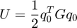
ureal = 0.5*q0'*G*q0;
for ia=1:numel(arange)
For each cutoff value, MSM is run to calculate the approximate force and potentials.
a=arange(ia);
Short-range Calculation
Here I prefer to create the matrices just to check the linear algebra side of the MSM match with the loop calculations.
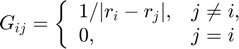
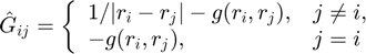
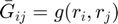
We split the G matrix into two parts:

where
    Ghat   = zeros(n,n);
    Gbar   = zeros(n,n);
    fshort = zeros(n,1);
I calculate the short-range potential in two ways: using the matrix algebra  and accumulating the potentials in the loop. That's why I use two different variables: ushort and ushortloop. In the end, I will compare them for sanity check.
    ushortloop = 0;
    for i=1:n
        qi = q0(i);
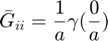

        Gbar(i,i) = s(0)/a;
        Ghat(i,i) = -Gbar(i,i);
        ushortloop = ushortloop + qi*qi*0.5*Ghat(i,i);
        for j=i+1:n
            qj     = q0(j);
            rij    = x0(i)-x0(j);
            r      = abs(rij);
            r_1    = 1/r;
            rij_r3 = rij/r^3;
            % Long-range
            if r >= a
                Gbar(i,j) = r_1;
                Gbar(j,i) = r_1;
                Ghat(i,j) = 0;
                Ghat(j,i) = 0;
            else
                % Short range
                g = s(r/a)/a;
                Gbar(i,j) = g;
                Gbar(j,i) = g;
                Ghat(i,j) = r_1-g;
                Ghat(j,i) = r_1-g;
                force = qi*qj*(1/r^2 + 1/a^2*sd(r/a))*rij/r;
                fshort(i) = fshort(i) - force;
                fshort(j) = fshort(j) + force;
                ushortloop = ushortloop + qi*qj*(r_1 - g);
            end
        end
    end
short-range potential energy is directly calculated by using
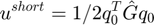
ushort = 0.5*q0'*Ghat*q0;
Anterpolation
Here I use similar strategy. I calculate the anterpolation matrix explicitly to check if the grid masses (q1) calculated by q1=A*q0 is equal to the grid masses (q1loop) calculated in the loop. Later, I will use A' in the interpolation step.
    nx1    = numel(x1);
    A      = zeros(nx1,n);
    q1loop = zeros(nx1,1);
    for i=1:n
        i0 = floor((x0(i)-x1(1))/h);
        t = (x0(i) - x1(i0))/h;
        A(i0  ,i) = c4(t);
        A(i0+1,i) = c3(t-1);
        A(i0+2,i) = c2(t-2);
        A(i0+3,i) = c1(t-3);
        q1loop(i0  ) = q1loop(i0  ) + c4(t  )*q0(i);
        q1loop(i0+1) = q1loop(i0+1) + c3(t-1)*q0(i);
        q1loop(i0+2) = q1loop(i0+2) + c2(t-2)*q0(i);
        q1loop(i0+3) = q1loop(i0+3) + c1(t-3)*q0(i);
    end
    q1 = A*q0;
Direct part (top level)
The matrix  is used to calculate the pairwise interactions between the grid masses q1.
    G1 = zeros(nx1,nx1);
    for i=1:nx1
        G1(i,i) = s(0)/a;
        for j=i+1:nx1
            r = abs(x1(j)-x1(i));
            if r >= a
                G1(i,j) = 1/r;
            else
                G1(i,j) = s(r/a)/a;
            end
            G1(j,i)=G1(i,j);
        end
    end
Grid potential e1 is just the matrix-vector product of G1 and q1.
e1 = G1*q1;
Interpolation
Since we already have the transformation matrix A in the anterpolation, I can use its transpose in the interpolation to get the long-range potentials in the particle level.
e0long = A'*e1;
I'll calculate the same e0long by using the loops to make sure I do the interpolation right.
e0longloop = zeros(n,1);
In the loop, I will calculate the long-range forces.
flong = zeros(n,1);
For each particle ...
    for i=1:n
        % Location of the particle
        x = x0(i);
        % lowest grid location having non-zero contribution.
        i0 = floor((x-x1(1))/h);
        % Coordinate of the particle in terms of h.
        t = (x - x1(i0))/h;
Sanity check: Since I'm using cubic bases, t should be between [1 2].
        if t < 1  || t > 2
            error('t should be between [1 2]');
        end
        flong(i) =  e1(i0  ) * c4d(t  )/h + ...
                    e1(i0+1) * c3d(t-1)/h + ...
                    e1(i0+2) * c2d(t-2)/h + ...
                    e1(i0+3) * c1d(t-3)/h;
        e0longloop(i) = e1(i0  ) * c4(t  ) + ...
                        e1(i0+1) * c3(t-1) + ...
                        e1(i0+2) * c2(t-2) + ...
                        e1(i0+3) * c1(t-3);
    end
Long-range potential energy is
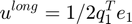
ulong = 0.5*q1'*e1;
Finally, I add the short and long-range energy and forces to obtain the final approximations.
    umsm = ushort+ulong;
    fmsm = fshort+flong;
Relative error in average mass-weighted force.
    errfunc = @(f,m) sqrt(mean((f.^2)./m));

    ferror(ia) = errfunc(freal-fmsm,q0)/errfunc(freal,q0);
Relative error in potential energy.
uerror(ia) = abs(ureal-umsm)/ureal;
Sanity checks
Short-range potential energies calculated two different ways should be equal to each other.
    if abs(ushort-ushortloop)/abs(ushort) > 1E-10
        error('ushort must be equal to ushortloop\n');
    end
Long-range potentials calculated by using both ways should be equal to each other.
    if norm(e0long-e0longloop)/norm(e0long) > 1E-10
        error('e0 should be equal to e0loop');
    end
The sum of grid masses should be equal to the total mass.
     if abs(sum(q0)-sum(q1))/sum(q0) > 1E-10
        error('sum(q0) should be equal to sum(q1)');
     end
The grid masses calculated both ways should be equal
    if norm(q1-q1loop)/norm(q1) > 1E-10
        error('q1 should be equal to q1loop');
    end
The long-range interaction kernel  is approaximated with the following relation.
If the particles are located on the grid nodes, then the approximation should be exact.
    Gtilde = A'*G1*A;
    if norm(Gbar-Gtilde)/norm(Gbar) > 1E-10
        error('The error in the approximation is high');
    end
Long-range potential energy can be calculated in two different ways. They should be equal.
    if abs(ulong-0.5*q0'*e0long) > 1E-10
        error('0.5*q0T*e0 shoulb be equal to ulong');
    end
end
The results
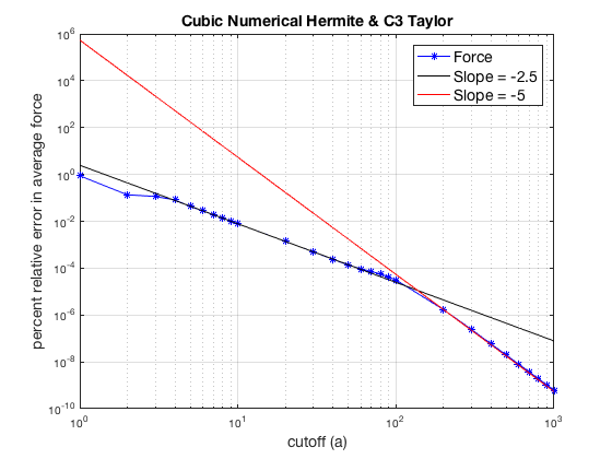
The percent relative error in average force is displayed in loglog plot. Here, I also plot two lines of slopes, -2.5 and -5, the later is for asymptotic behaviour. The expected slopes are -4 and -5 since I'm using cubic (p=3) interpolating polynomials. But the observations in the dissertation and my experiments with NAMD-Lite indicates that we should observe -3 and -5. However, my code produces a slope -2.5. I'm still not sure why I can't get a slope of -3.
loglog(arange,ferror,'b-*');
hold on
loglog(arange,(ferror(10)*arange(10)^2.5)*arange.^-2.5,'k-');
loglog(arange,(ferror(20)*arange(20)^5)*arange.^-5,'r-');
title('Cubic Numerical Hermite & C3 Taylor','FontSize',14);
xlabel('cutoff (a)','FontSize',14);
ylabel('percent relative error in average force','FontSize',14);
h=legend('Force','Slope = -2.5','Slope = -5');
set(h,'FontSize',14);
grid on
set(gcf,'color','w');
export_fig('matlab_grid_Cubic_C3Taylor.pdf');